R project (Air pollution)

Here you will be able to see a project made with the programming language R.

In this project I will analyze the air pollution and meteorological data from 1991 to 2021 in my city, Martorell .

1. Data collection:

• The data can be found by googling "open data atmosphere" and "meteocat open data":
• Air pollution data
• Meteorological data
• We must take into account that the data are hourly for pollution and the meteorological data are semi-hourly (every 30 minutes) that we have to combine in a single dataframe to make graphs that relate both types of data. The weather data will be from the station closest to our pollution station.
• From the meteorological data the codes of the variables that we need are 30 for wind speed that we will put ws, and 31 for wind direction that we will put wd. The dates will be in ISO8601 format 2021-03-15 16:00:00 with POSIXct format with the name date. The names date, ws and wd are Openair requirements.

2. Required software:

• RStudio software and the Tidyverse and Openair packages must be installed.
• Tidyverse allows you to sort the data.
• Openair allows hour by hour, day by day, year by year air studies in a specific and advanced way.
• To install these 2 R packages you must type:

  install.packages (c("tidyverse","openair"))

3. Sorting the atmospheric data:

• We must read the data from our computer:

city<-read.csv("C://Users/YOURCOMPUTERNAME/Documents/city.csv")

View(city)

• We change the times of the columns to rows

city1<-pivot_longer(city,cols=c(h01,h02,h03,h04,h05,h06,h07,h08,h09,h10,h11,h12,h13,h14, h15,h16,h17,h18,h19,h20,h21,h22,h23,h24), names_to="hour", values_to = "value")

city2<-city1[-c(1,2,4,6:16)]

write.csv(city2,"C:\\Users\\YOURCOMPUTERNAME\\Documents\\city2.csv")

4. Modify the atmospheric data (with LibreOffice Calc or Visual Studio Code):

• We delete T00.00.00.000 and replace the times H01, etc for 01:00:00 until we get the dates in ISO format:

• We associate date and time together to city4.csv using LibreOffice Calc or RStudio.

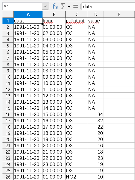
city4 <- city3 %>% mutate(name=paste0(data, " ", hour))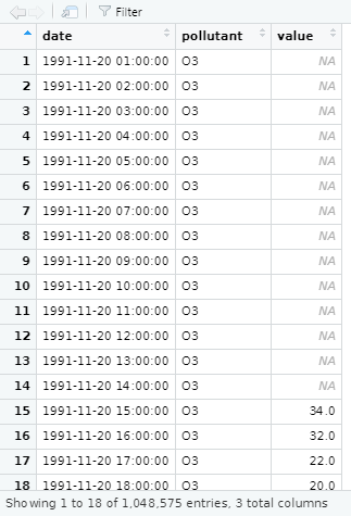

• We create city5 by putting day and time together under the column name date


5. Converting the data format:

library(openair)

city5PM10 <- subset(city5, pollutant=="PM10")

city5PM10$date<-as.POSIXct(city5PM10$date,"%Y-%m-%d %H:%M:%S", tz="Europe/Madrid")

class(city5PM10$date)

The answer has to be:

[1] "POSIXct" "POSIXt"

View(city5PM10)

It is important to ensure that the date is not a character set but a POSIX, a data.

class(city5PM10$date)

The answer will be:

[1] "character"

So we have to change it to a POSIXct

city5PM10$date<-as.POSIXct(city5PM10$date,"%Y-%m-%d %H:%M:%S", tz="Europe/Madrid")

class(city5PM10$date)

The answer has to be:

[1] "POSIXct" "POSIXt"

class(city5PM10$pollutant)

The answer will be:

[1] "character"

So we have to change it to a factor

city5PM10$pollutant<-as.factor(city5PM10$pollutant)

class(city5PM10$pollutant)

The answer has to be:

[1] "factor"

6. Sorting the data with pivot_wider:

library(tidyverse)
library (openair)
city6<-pivot_wider(city5, names_from= pollutant, values_from =value)
View (city6)
write.csv(city6,"C:\\Users\\YOURCOMPUTERNAME\\Documents\\MYCITY\\city6.csv")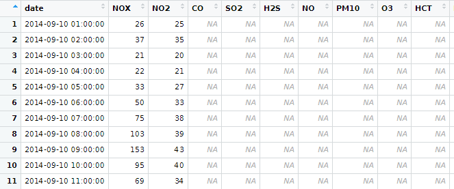



7. Creating graphs with Openair R:

7.1 Time Variation:

timeVariation(city5PM10, pollutant="value")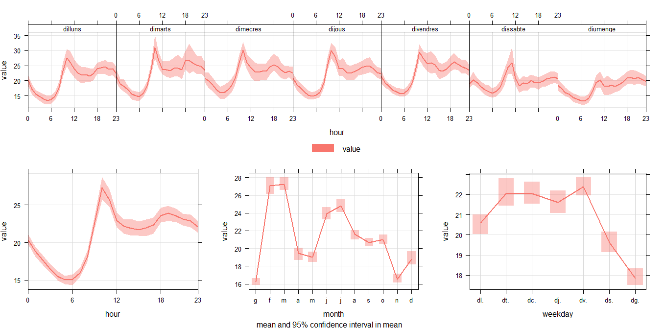



7.2 Trend Level:

trendLevel(city5PM10, pollutant = "value", main="PM10 evolution in MYCITYNAME")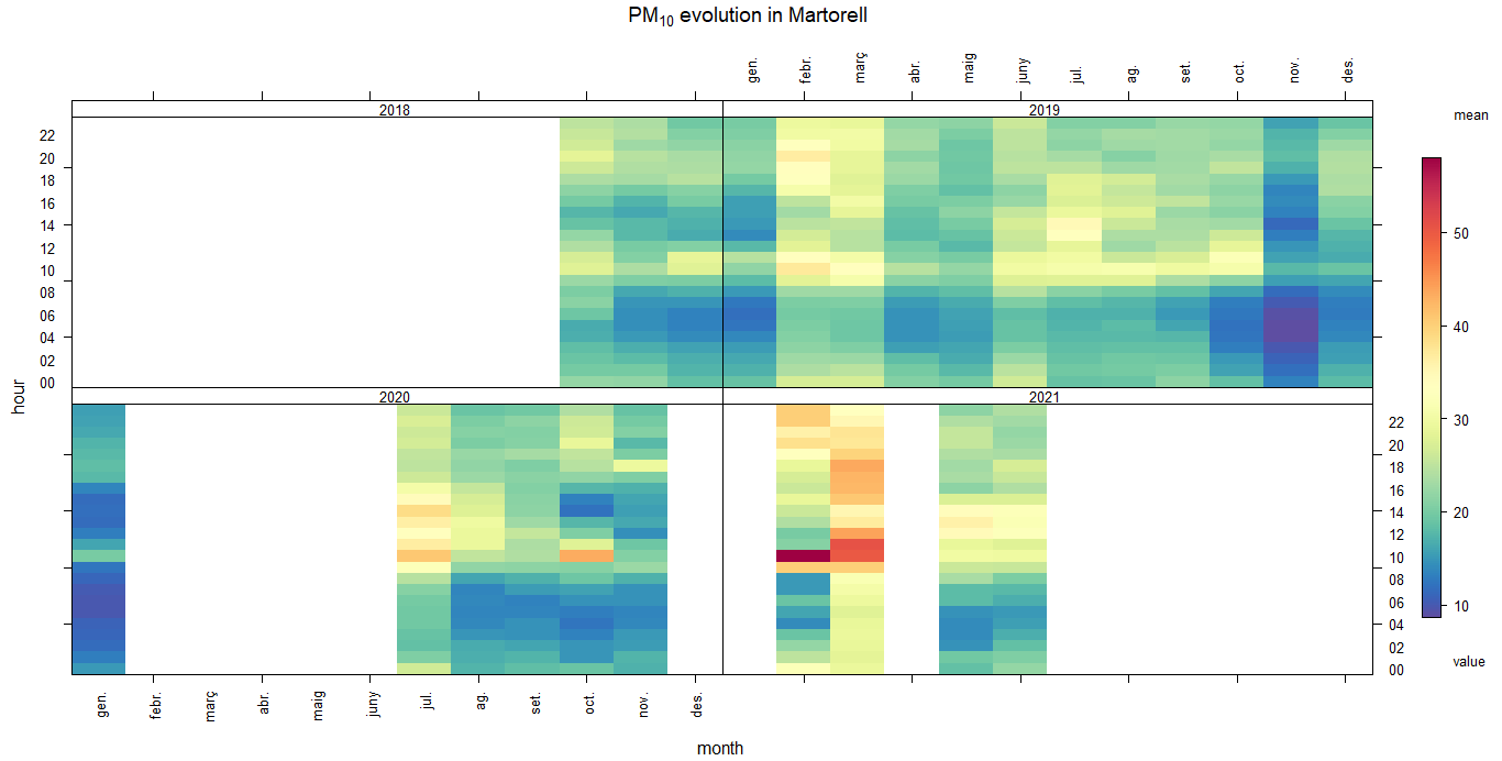



7.3 Calendar Plot:

daily<-timeAverage(city5NO2,avg.time = "day")
View(daily)
calendarPlot(city%NO2, pollutant="value", year="2020")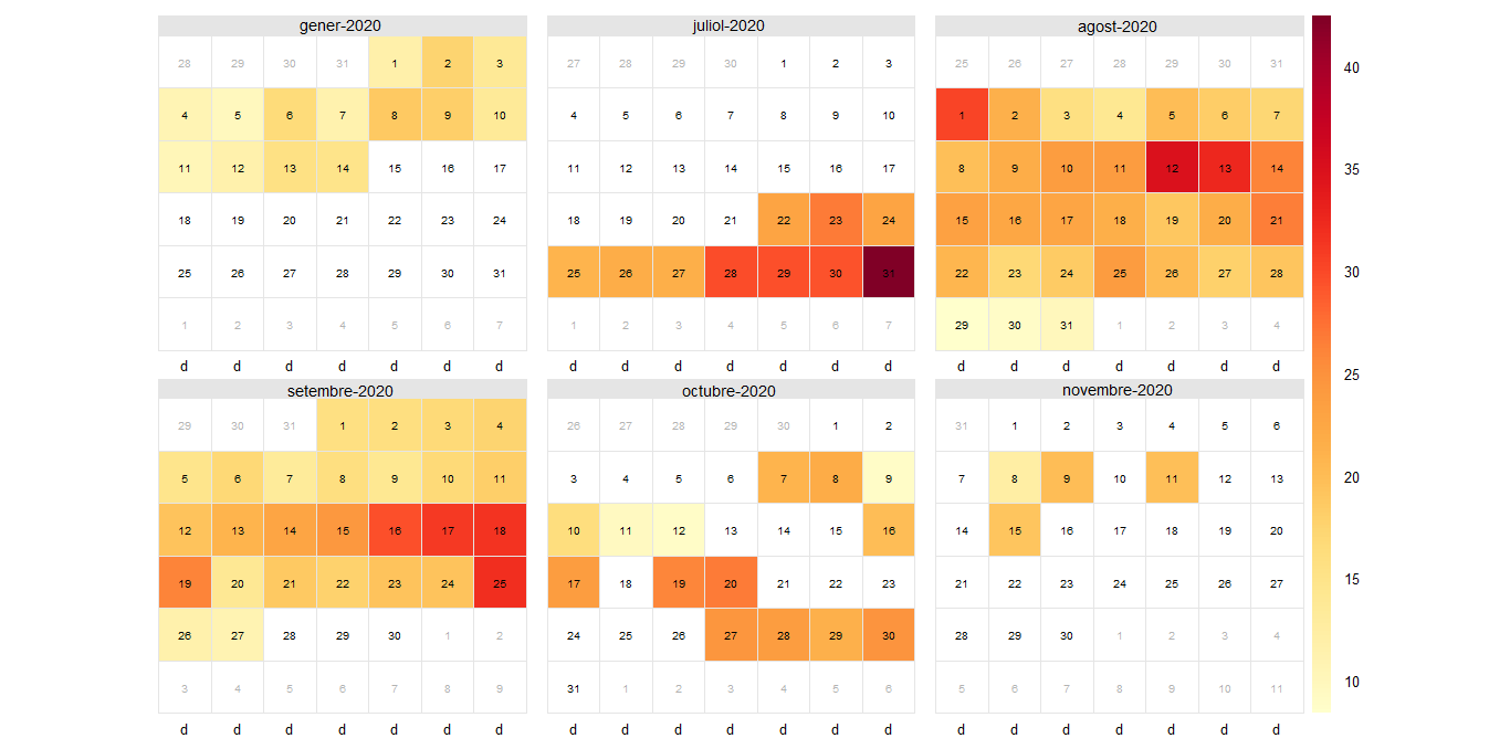



7.4 Yearly:

yearly<-timeAverage(city5NO2,avg.time = "year")
View(yearly)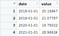



7.4.1 Summary Plot:

summaryPlot(yearly)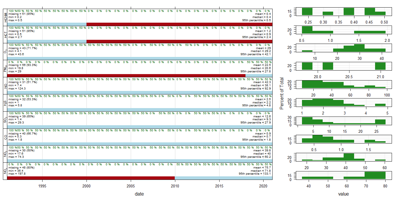



7.4.2 Time Plot (yearly):

timePlot(selectByDate(yearly), pollutant = c("NOX","NO2","CO","SO2","H2S","NO","PM10","O3", "HCT","HCNM"), y.relation = "free", main="Yearly mean of air pollutants in MYCITYNAME")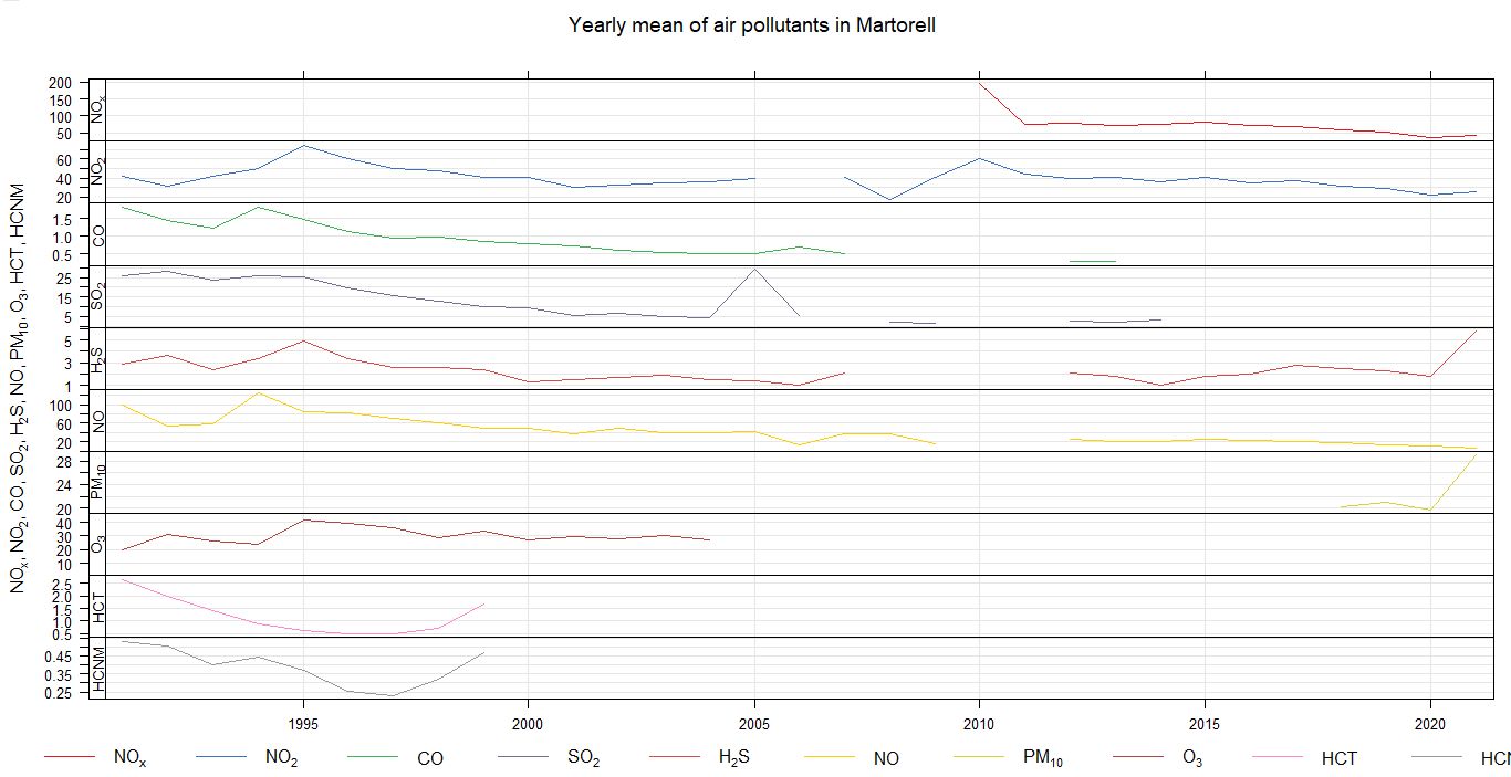



7.4.3 Time Plot (city6):

timePlot(selectByDate(city6), pollutant = c("NOX","NO2","CO","SO2","H2S","NO","PM10","O3", "HCT","HCNM"), y.relation = "free", main="Yearly mean of air pollutants in MYCITYNAME")



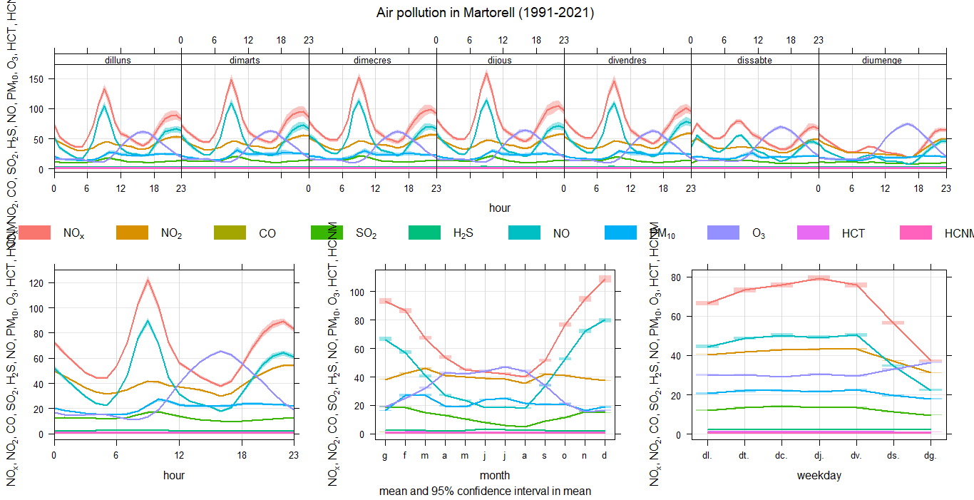
7.5 Time variation of pollutants 1991-2021:

class(city6$date)

The answer will be:

[1] "character"

So we have to change it to a POSIXct

city6$date<- as.POSIXct(city6$date,format="%Y-%m-%d %H:%M:%S",tz="Europe/Madrid")
timeVariation(city6, pollutant=c("NOX","NO2","CO","SO2","H2S","NO","PM10","O3", "HCT","HCNM"), main="Air pollution in MYCITY (1991-2021)")



Episode (extra):

• Air quality standards indicate different pollution limit levels,for example, for NO2; levels must be below 40 µg/m3.
• We can check for example the number of exceedances of the eight-hour ozone averages with this code:

library(openair)
episode<-selectRunning(city6, pollutant="O3",threshold=120, run.len=8)
nrow(episode)

In this case, the answer is:

[1] 95

The program tells us that the level of 120 µg/m3 has been exceeded in the 8h average a total of 95 times.

8. Sorting weather data:

wind<-read.csv("C://Users/YOURCOMPUTERNAME/Documents/wind.csv")

View(wind)

wind1<-wind[-c(1,2,5,7,8)]

wind2<-pivot_wider(wind1,names_from = CODI_VARIABLE, values_from = VALOR_LECTURA)

names(wind2)[names(wind2) == "31"] <- "wd"

names(wind2)[names(wind2) == "30"] <- "ws"

names(wind2)[names(wind2) == "DATA_LECTURA"] <- "date"

write.csv(wind2,"C:\\Users\\YOURCOMPUTERNAME\\Documents\\wind2.csv")

9. Linking the two databases (pollutants and meteo):

The data we downloaded from the meteorology database indicated in the previous section are semi-hourly and expressed in AM and PM and we need to proceed with Calc's Find and Replace or Visual Studio Code so that it has the same format as the pollution data.



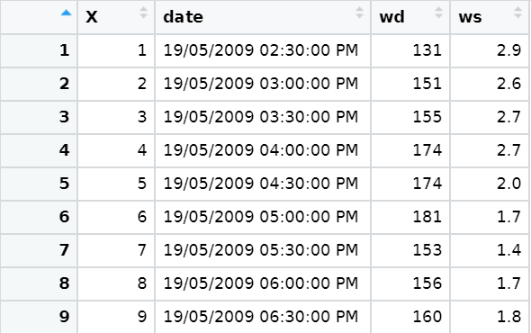
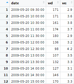
We create the hourly data from half-hours:

• 1º way of doing it:

  library (openair)
  wind3<-timeAverage(wind2, time.avg="hour")

• 2º way of doing it:

  toDelete <- seq(2, nrow(wind2), 2)
  wind3<-wind2[ toDelete ,]

We have to be sure that the wind database date class is a POSIXct date type in order to combine it.

It can be joined with different instructions, for example, with one of Openair:

cityall<-merge(city6, wind5, by ="date")
View (cityall)



9.1 Pollution Rose:

And now we can do pollutionRose and see where the pollution is coming from.

pollutionRose(cityall, pollutant = "PM10")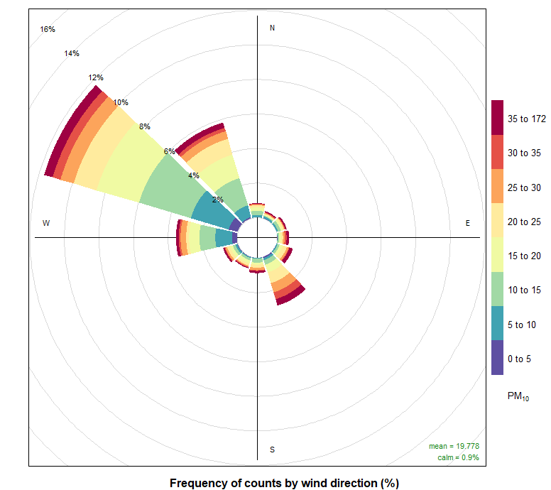



10. Conclusions:

With all the data that we have collected we could see If there are some values that exceed the legal limit of pollution and with the wind graphic (Pollution Rose) we could see where does the pollution come from.

The graphics are a good way to detect that high values of pollution and I think that this has been a good introduction into R language and a good way to learn basic code with RStudio as It has been very practic to work for the time with a large number of data.